A more complex/realistic example demonstrating how parakat can be used to speed up 2-dimentional simulations is provided at the end of this post.
The example Finesse code used in Parallelising Finesse 2 + PyKat: three ways is deliberately simple and quick so we can demonstrate some basic functionality. However it’s not a situation you’d realistically encounter, or one that would likely motivate you to try parallelising your code in the first place.
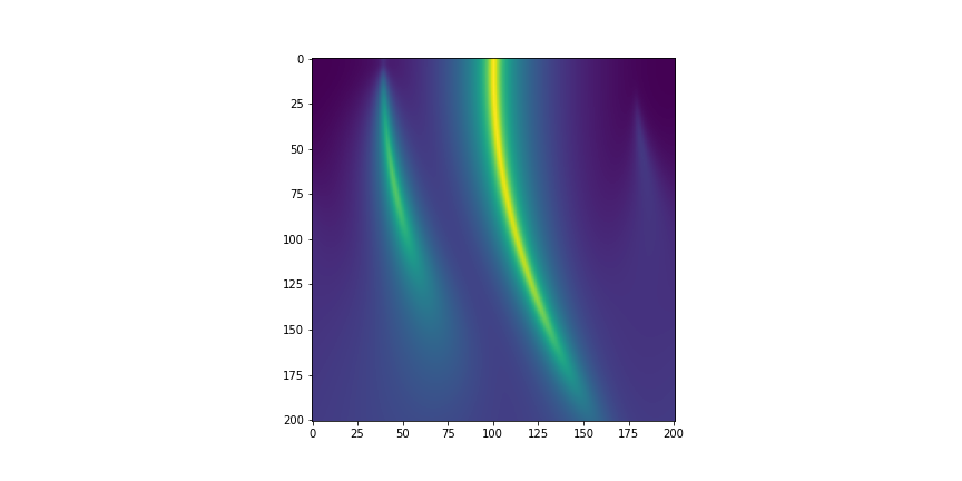
In this example, the user wanted to model a 2-mirror cavity that has a slightly misaligned input mirror (therefore requiring the use of higher order modes). They are interested in understanding how the cavity resonant conditions change with this misalignment, so want to compare cavity scans (circulating power as a function of cavity tuning) as the value of the misalignment is varied.
The base Finesse code, parsed directly to Pykat, is:
base = finesse.kat()
base.verbose=False
base.parse("""
l L0 1 0 n0
s s0 0 n0 n1
m m1 0.95 0.05 0 n1 n2
s s1 100 n2 n3
m m2 0.95 0.05 0 n3 n4
attr m2 Rc 150
attr m2 xbeta 1u
cav c1 m1 n2 m2 n3
pd pow n2
maxtem 3
""")
NB: as-written, this example uses maxtem 3 and few (80) steps along each axis, so that it runs quite fast for demonstration purposes. it will quickly get a lot slower when these numbers are increased, as you would likely need to do for a more complete and accurate understanding of the result.
Standard, non-parallel method
Finesse can handle multiple x-axes commands. It does this in series by scanning the parameter of the xaxis for each x2axis value in sequence. The syntax is simply:
kat = base.deepcopy()
kat.parse("""
xaxis m2 phi lin -90 90 80
x2axis m1 xbeta lin 0 80u 80
""")
out = kat.run()
which will directly (eventually) produce a 2D output object out["pow"], along with a list of the input parameter choices in out.x and out.y [check!] for the xaxis and x2axis parameters respectively, that can be plotted however you like.
Using parakat to speed things up
We can speed this up by instead just calculating the xaxis and splitting the x2axis into chunks that run in parallel on different engines.
Using ipcluster via subprocess we first start 8 engines:
n_eng = 8 # max number of parallel tasks

subprocess.run(f"ipcluster start -n {n_eng} --daemonize",shell=True)
time.sleep(10) # wait a few sec for the cluster to start up
Then set up the equivalent of the x2axis command above, using a for-loop to create each kat object we’ll need and distribute these between the 8 engines:
xstart = 0
xstop = 80e-6
xpoints = 201
xaxis = np.linspace(xstart,xstop, xpoints) #equivalent to x2axis above
sp = np.array_split(xaxis,n_eng) #separate this into 8 smaller sections that run simultaneously

pk = parakat()
for T in np.arange(n_eng):
    kat = base.deepcopy()
    kat.parse("xaxis m2 phi lin -90 90 200") #same as before
    kat.parse(f"x2axis m1 xbeta lin {sp[T][0]}  {sp[T][-1]} {len(sp[T])-1}") # sub-section of old x2axis
    pk.run(kat)
outs = pk.getResults()

# Stopping the cluster
subprocess.run(f"ipcluster stop",shell=True)
time.sleep(3) #wait a sec for the cluster to shut down
This time, we have to manually merge our 8 pieces of output data back into one plot:
def twod(b):
    # reducing output data from 3D array (1,n,m) to 2D array (n,m)
    #print(np.shape(b))
    return np.reshape(b, (b.shape[1], b.shape[2]))

x = outs[0].x
y = xaxis
data = twod(outs[0].z)
for T in np.arange(1,n_eng):
    #print(T)
    data = np.vstack([data,twod(outs[T].z)])
Now, as before, we can use the final 2D object called data, along with full input parameter lists x and y, to plot the data as we want.
fig, ax = plt.subplots(1,1, figsize=(12,6))
ax.imshow(data, norm=LogNorm(), aspect='equal')