I used fenicsx to create stress simulations of a silicon test mass which could then be converted to birefringence. The model used was based on the silicon test masses created for use in the Gingin 7m 2um cavity project. These have a diameter of 10cm and a thickness of 3cm. All the values used in the code are in SI units. Gravity acts in the negative z direction and the optical axis is the x direction. I created the mesh using the python api for gmsh and then imported it into dolfinx
from mpi4py import MPI
from dolfinx.io.gmshio import model_to_mesh
import pyvista
from dolfinx import mesh, fem, plot, io, default_scalar_type
from dolfinx.fem.petsc import LinearProblem
from mpi4py import MPI
import ufl
import numpy as np
import gmsh
import warnings
warnings.filterwarnings("ignore")
gmsh.initialize()

gmsh.model.add("test_mass")
cad = gmsh.model.geo
lc = 0.002
cad.addPoint(0, -0.05, 0.01, lc, 1)
cad.addPoint(0, 0.05, 0.01, lc, 2)
cad.addPoint(0, 0.05, -0.01, lc, 3)
cad.addPoint(0, -0.05, -0.01, lc, 4)
cad.addPoint(0,0,0, lc, 5)
cad.addLine(2, 3, 1)
cad.addLine(4, 1, 2)
cad.addCircleArc(1, 5, 2, 3)
cad.addCircleArc(3, 5, 4, 4)
cad.addCurveLoop([3, 1, 4, 2 ], 10)
cad.addPlaneSurface([10], 11)
vol = cad.extrude([(2, 11)], 0.03,0,0 )
cad.synchronize()
gmsh.model.addPhysicalGroup(3, [vol[1][1]], 41, "volume")
gmsh.model.addPhysicalGroup(2, [vol[0][1],vol[2][1], vol[3][1], vol[4][1], vol[5][1]], 42, "surface")
gmsh.model.mesh.generate(3)
model_rank = 0
domain, cell_tags, facet_tags = model_to_mesh(
    gmsh.model, MPI.COMM_WORLD, model_rank,3)
I then used dolfinx to run the finite element analysis. This produces a measurement of the deformation of each element. I set the boundary conditions so that the flat edges of the test mass were fixed. The code for the linear elasticity calculation is based on this dolfinx tutorial: https://jsdokken.com/dolfinx-tutorial/chapter2/linearelasticity_code.html
E = 130e9
nu = 0.27
mu = E / (2.0 * (1.0 + nu))
lambda_ = E * nu / ((1.0 + nu) * (1.0 - 2.0 * nu))
rho = 2329
g = 9.8
V = fem.VectorFunctionSpace(domain, ("Lagrange", 1))
def clamped_boundary(x):
    return np.logical_or(np.isclose(x[1], -0.05), np.isclose(x[1], 0.05))


fdim = domain.topology.dim - 1
boundary_facets = mesh.locate_entities_boundary(domain, fdim, clamped_boundary)
u_D = np.array([0, 0, 0], dtype=default_scalar_type)
bc = fem.dirichletbc(u_D, fem.locate_dofs_topological(V, fdim, boundary_facets), V)
T = fem.Constant(domain, default_scalar_type((0, 0, 0)))
ds = ufl.Measure("ds", domain=domain)
def epsilon(u):
    return ufl.sym(ufl.grad(u))  # Equivalent to 0.5*(ufl.nabla_grad(u) + ufl.nabla_grad(u).T)


def sigma(u):
    return lambda_ * ufl.nabla_div(u) * ufl.Identity(len(u)) + 2 * mu * epsilon(u)


u = ufl.TrialFunction(V)
v = ufl.TestFunction(V)
f = fem.Constant(domain, default_scalar_type((0, 0, -rho * g)))
a = ufl.inner(sigma(u), epsilon(v)) * ufl.dx
L = ufl.dot(f, v) * ufl.dx + ufl.dot(T, v) * ds
problem = LinearProblem(a, L, bcs=[bc], petsc_options={"ksp_type": "preonly", "pc_type": "lu"})
uh = problem.solve()
The deformation can then be plotted in pyvista which gives:
pyvista.start_xvfb()

# Create plotter and pyvista grid
p = pyvista.Plotter()
topology, cell_types, geometry = plot.vtk_mesh(V)
grid = pyvista.UnstructuredGrid(topology, cell_types, geometry)

# Attach vector values to grid and warp grid by vector
grid["u"] = uh.x.array.reshape((geometry.shape[0], 3))
#actor_0 = p.add_mesh(grid, style="wireframe", color="k")
warped = grid.warp_by_vector("u", factor=1.5)
actor_1 = p.add_mesh(warped, show_edges=False)
p.show_axes()
if not pyvista.OFF_SCREEN:
    p.show()
else:
    figure_as_array = p.screenshot("deflection.png")
Now we have to convert from the deformation to the stress tensor by interpolating onto a new vector function space. This gives the flattened list of the stress tensor components for each element. This is reshaped into a 3×3 tensor.
gdim = domain.geometry.dim
Stress = fem.VectorFunctionSpace(domain, ("Discontinuous Lagrange", 0, (gdim,)), 9)
stress = fem.Function(Stress)
stress_expr = fem.Expression(sigma(uh), Stress.element.interpolation_points())
stress_array = stress.x.array.reshape((int(stress.x.array.shape[0]/9), 3, 3))
Next we define the functions to calculate the birefringence. The calculation for the stress induced birefringence first calculates the change in the inverse dielectric tensor (optical index ellipsoid) and then calculates the eiegenvalues of the rotated tensor. The eigenvalues can then be used for a calculation of the birefringence.
def rot_mat(rot_z, rot_y, rot_x):
    a = rot_z
    b = rot_y
    y = rot_x
    mat = np.array([[np.cos(a)*np.cos(b), np.cos(a)*np.sin(b)*np.sin(y) - np.sin(a)*np.cos(y), np.cos(a)*np.sin(b)*np.cos(y) + np.sin(a)*np.sin(y)],[np.sin(a)*np.cos(b), np.sin(a)*np.sin(b)*np.sin(y) + np.cos(a)*np.cos(y), np.sin(a)*np.sin(b)*np.cos(y) - np.cos(a)*np.sin(y)], [-1*np.sin(b), np.cos(b)*np.sin(y), np.cos(b)*np.cos(y)]])
    return mat


def h_eigenvalues(mat):
    a = mat[0, 0]
    b = mat[1, 1]
    c = mat[0, 1]

    l1 = (a + b - np.sqrt(4 * c ** 2 + (a - b) ** 2)) / 2
    l2 = (a + b + np.sqrt(4 * c ** 2 + (a - b) ** 2)) / 2
    return l1, l2


def r_index(mat):
    l1, l2 = h_eigenvalues(mat)
    return (1/np.sqrt(l1)) - (1/np.sqrt(l2))


def stress(s1, s2, s3, s4, s5, s6):
    arr = np.array([s1, s2, s3, s4, s5, s6])
    return arr


def photoelastic(p11, p12, p44):
    arr = np.array([[p11, p12, p12, 0, 0, 0], [p12, p11, p12, 0,0,0], [p12, p12, p11, 0,0,0],[0,0,0,p44,0,0],[0,0,0,0,p44,0],[0,0,0,0,0,p44]])
    return arr


def elastic(PR, YM):
    arr = np.array([[1, -1*PR, -1*PR,0,0,0],[-1*PR, 1, -1*PR, 0,0,0], [-1*PR, -1*PR, 1,0,0,0],[0,0,0,1+PR,0,0],[0,0,0,0,1+PR,0],[0,0,0,0,0,1+PR]])
    arr = arr * (1/YM)
    return arr


def delta_b(PR, YM, p11, p12, p44, s1, s2, s3, s4, s5, s6):
    arr = np.dot(photoelastic(p11, p12, p44), np.dot(elastic(PR, YM), stress(s1, s2, s3, s4, s5, s6)))
    return arr


def b_0(nx, ny, nz):
    arr = np.array([1/(nx**2), 1/(ny**2), 1/(nz**2), 0,0,0])
    return arr


def b_new(PR, YM, s1, s2, s3, s4, s5, s6, p11, p12, p44, nx, ny, nz):
    delB = delta_b(PR, YM, p11, p12, p44, s1, s2, s3, s4, s5, s6)
    B0 = b_0(nx, ny, nz)
    B = delB + B0
    arr2 = np.array([[B[0], B[5], B[4]], [B[5], B[1], B[3]], [B[4], B[3], B[2]]])
    return arr2


def birefringence(rot_z, rot_y, rot_x, PR, YM, s1, s2, s3, s4, s5, s6, p11, p12, p44, nx, ny, nz):
    b = b_new(PR, YM, s1, s2, s3, s4, s5, s6, p11, p12, p44, nx, ny, nz)
    rot = rot_mat(rot_z, rot_y, rot_x)
    rotated = np.dot(rot, np.dot(b, np.linalg.inv(rot)))
    small_b = rotated[1:, 1:]
    delta_n = r_index(small_b)
    return delta_n
Now we just have to find the birefringence for each element in the interpolated mesh. The first three elements of the birefringence function are the rotation of the optic around the z, x and y axes. The next two are the Poisson ratio and the Young’s modulus of silicon. The next six are the elements of the stress tensor in voigt notation. Then the next three are the non-zero elements of the photoelastic tensor for cubic crystals. The last three are the refractive indicies in the x, y and z direction.
npoints = stress_array.shape[0]
dn = np.zeros(npoints)
for x in range(npoints):
    a = stress_array[x]
    dn[x] = birefringence(rot_z=0, rot_x=0, rot_y=0, PR=0.27, YM=130e9, s1=a[0,0], s2=a[1,1], s3=a[2,2],s4= a[1,2], s5=a[0,2],s6=a[0,1], p11=-0.094, p12=0.017,p44= -0.051, nx=3.48, ny=3.48, nz=3.48)
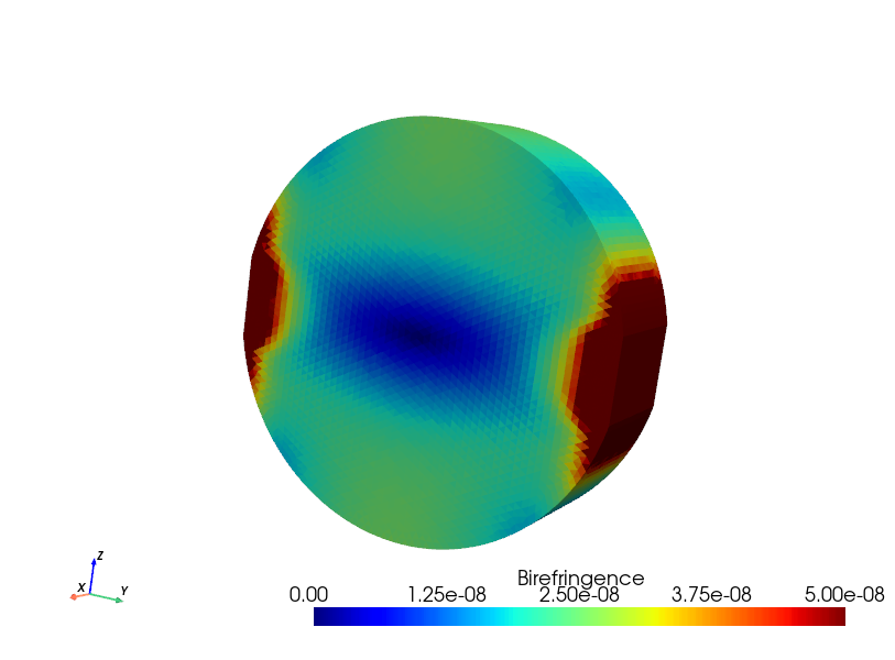
Having calculated the birefringence we can now plot it onto the mesh. The simulation of birefringence gives a result comparable with past measurements (https://dcc.ligo.org/LIGO-P2200357).
pyvista.global_theme.cmap = 'jet'
warped.cell_data["Birefringence"] = dn
warped.set_active_scalars("Birefringence")
p = pyvista.Plotter()
p.add_mesh(warped, clim=[0, 5e-8])
p.show_axes()
if not pyvista.OFF_SCREEN:
    p.show()
else:
    stress_figure = p.screenshot(f"stresses.png")