Note: This post is based on the relevant Finesse 3 documentation page: https://finesse.docs.ligo.org/finesse3/usage/homs/selecting_modes.html
Models in Finesse are, by default, created as plane-wave representations of the underlying configuration. This can be switched to a modal basis by specifying the mode indices that should be modelled by the system. There are a few key ways in which this can be done, as outlined in the sections below.
Maximum TEM order
The maximum TEM order (termed maxtem for short) is something that will be familiar for users of previous Finesse versions. By setting a value for maxtem, all mode indices up to and including this order will be included in the model. For example:
import finesse

model = finesse.Model()
# set maximum mode order (n+m) to 3
model.select_modes(maxtem=3)

print(model.homs)
will produce the output:
[[0 0]
 [0 1]
 [0 2]
 [0 3]
 [1 0]
 [1 1]
 [1 2]
 [2 0]
 [2 1]
 [3 0]]
This can also be achieved via the finesse file syntax with:
modes maxtem=3Selection method
One of the main new features of modelling HOMs in Finesse 3 is the ability to select the modes you want to model rather than including all modes up to a specific order with maxtem. This can be achieved via varied arguments to the Model.select_modes() method. Below are a few examples, with both the Python API and parsed syntax representations given.
Even modes up to order 4
model.select_modes("even", 4)modes even maxtem=4Modes in the model:
[[0 0]
 [0 2]
 [0 4]
 [2 0]
 [2 2]
 [4 0]]
Odd modes up to order 3
model.select_modes("odd", 3)modes odd maxtem=3Modes in the model:
[[0 0]
 [0 1]
 [0 3]
 [1 0]
 [1 1]
 [3 0]]
Tangential modes up to order 5
model.select_modes("x", 5)modes x maxtem=5Modes in the model:
[[0 0]
 [1 0]
 [2 0]
 [3 0]
 [4 0]
 [5 0]]
Sagittal modes up to order 4
model.select_modes("y", 4)modes y maxtem=4Modes in the model:
[[0 0]
 [0 1]
 [0 2]
 [0 3]
 [0 4]]
Mode selection in practice
The example below shows a file with the input laser L0 mismatched to the the cavity eigenmode. As there are no misalignments in this system, we can ignore any odd modes and just model even modes.
import finesse
finesse.init_plotting()

model = finesse.Model()
model.parse("""
l L0 P=1
s s0 L0.p1 ITM.p1

m ITM R=0.99 T=0.01 Rc=-2.5
s sCAV ITM.p2 ETM.p1 L=1
m ETM R=0.99 T=0.01 Rc=2.5

# create the cavity object
cav FP ITM.p2.o
# make a mismatch by setting a different propagated q at laser
gauss gL0 L0.p1.o q=-0.7+0.9j

# only care about even modes as we're just looking
# at mismatches, so select even modes up to order 4
modes even 4

pd transmitted_power ETM.p2.o

xaxis ETM.phi lin -180 180 500
""")

out = model.run()
out.plot(logy=True)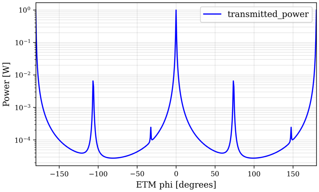
From this plot you can see that we get the scattering into 02 and 04 modes as expected from introducing a mode-mismatch.
Note that for this small example, the speed-up from only modelling even modes is not particularly noticeable for users. However, even for small configurations such as this simple cavity model the performance improvement when selecting the “right” modes will be significant when going to higher maxtem values and when scanning over a degree of freedom which results in different scattering matrices at each data point. A future logbook post or documentation page will quantify the amount of performance improvements achieved from this.
Very nice example and comment.
BTW why do you use the second output argument (‘_’) in the line `figures, _ = out.plot(logy=True)`
The plotting function currently returns a dictionary of figures and a dictionary of animations. I just realised, however, that I can change this to just return the figures if the animations dict is empty. I’ll make that change to the plot function soon.
Of course, in this example the figures dict isn’t really needed either – it was just left in as I used it to save the plot shown.